
Machine instructions can be used in routines either to make an inner loop more efficient or to effect some operation which cannot easily be done otherwise. It is assumed that the reader is reasonably familiar with the logical structure of the machine, that is with the basic order code. It also essential to know how data is stored in the stack. We illustrate this with reference to the following routine.
routine matrix fn (array name A,B integer m,n real fn F)
real a,b,c ;  integer i,j
array C(1:m,1:n),E(1:m)
real fn spec F (real x)
---
---
cycle i = 1,1,m
cycle j = 1,1,n
---
---
repeat
repeat
--
--
end
1. The first word of the local stack section contains the control number for returning to the calling routine (the first half word) and the previous contents of Bd, the current level B-line (the second half word). The 1st half word of the second word contains the test link (which records the position within the label list of a test instruction), and the 2nd half word contains information ( the number and type of the routine and the number of fixed variables) required by the run-time fault monitor routine. Here Bd refers to the B-line associated with the routine, and corresponds to the textual depth of the routine in the program in which it is embedded. If (say) this is 2 then Bd ≡ B2. The relative locations of the fixed variables A, B, m, n etc., are assigned at compile time. Immediately on entry to the routine the current value of B90, which always points to the next available location in the stack, is recorded in Bd and the previous contents of Bd recorded in the stack (as already noted). B90 is then advanced to the end of the fixed storage allocation. When the declarations for C and D are 'obeyed' it is advanced again to the final value shown.
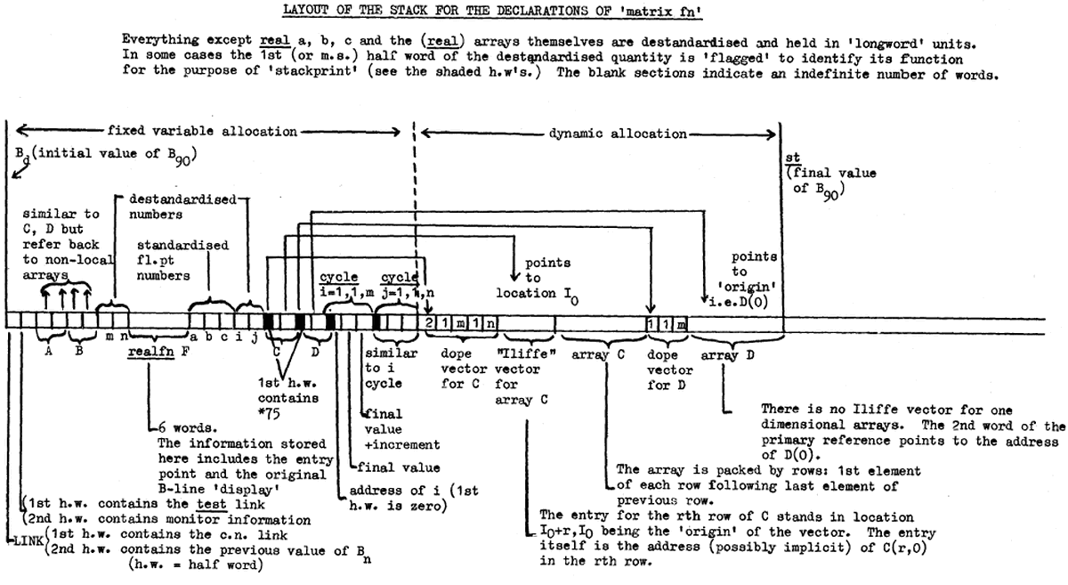
2. Destandardised quantities are formed by adding 0*8↑(-12) to the standardised form. This constant will be found in location *1000001. This octal form of the address can be used in machine instruction formats(see later). There are no integer name or real name parameters in this example; if present they would be represented (at the appropriate place among the fixed variables) by single words, namely their addresses, in a destandardised form. They are at present in distinguishable from integer's. Similarly for complex name parameters. A complex quantity requires two consecutive words, representing the real and imaginary parts.
3. ARRAYS. The primary reference to an array consists of a pair of words. The second half of the 1st word points to the (1st word of the) 'dope vector', that of the second word to the 'Iliffe vector'. The dope vector contains the values of the bound-pair list together with the number of pairs, i.e. the dimensionality of the array. If there is more than one array associated with same bound-pair list they share the same dope vector. The Iliffe vector gives the origin of each row of the matrix (which is stored by rows). The purpose of this is to simplify computation involved in accessing an element of the array. Thus for example to add C(i+5,j-6) into the accumulator the instructions are:-
    101, 96, d, i + ½       put i in β96
    104, 96, 0, c + 1½      β96 = β96 + 10
    101, 97, d, j + ½       put j in β97
    104, 97, 96, 5½         β97 = β97 + entry for row (i+5)
    320, 0, 97, -6          acc = acc + real (β97 - 6)
Similarly to add the element D(i+5) of the one-dimensional array D (which has no Iliffe vector) one may write
    101, 97, d, i + ½       put i in B97
    104, 97, 0, D + 1½      B97 = B97 + addr (D(0))
    320, 0, 97, 5           acc = acc + real (B97 + 5)
In these instructions i, C, j, D refer to the addresses of these quantities (see later)
Arrays of k dimensions (>2) are stored in hierarchical fashion. The primary Iliffe vector points to a set of arrays of k - 1 dimensions stored end to end. Each such array consist of an Iliffe vector referring to a set of k - 2 dimensional arrays, and so on.
4. THE PARAMETRIC FUNCTION F. Six words of information are kept here. In addition to the control number for entering the routine it is necessary to keep a record of the display of the relevant B-lines when the routine is first substituted as an actual parameter. For further details see the Compiler.
5. THE CYCLES. As explained in the text the initial and final values and increment in a cycle are evaluated and checked for compatibility before the cycle is commenced. The increment and final values, together with the address of the controlled integer variable are recorded for use in the execution of the cycle. The diagram illustrates how they are stored.
The following autocode formats involving the stack pointer (B90) are available
st = st ± [EXPR']
st =  [EXPR]
[NAME] = st
st represents the contents of B90. In the last instruction the [NAME] must be local to the routine containing the instruction, otherwise a fault is indicated.
Some 'machine code' formats are now described.
1. Where there is no symbolic address involved an instruction is written in the form
[FD],[N],[N],[ADDRESS PART]
(and terminated as usual by ; or newline). Here [FD] refers to the function digits, [N] to the Ba and Bm digits, and [ADDRESS PART] to the address part, which may take a number of forms. It may be written as a constant in the usual way (preceded possibly by a sign) bearing in mind that the binary point is located 3 places from the right hand end. Thus
    0121, 80, 0, 2.5     is equivalent to
    05064000  00000024
It may also consist of an octal number which consists of an * followed by up to 8 octal digits, including any significant zeros. Thus
    O101, 91, 0, *1001     is equivalent to
    04066600  10010000
in octal notation.
Finally it may consist of a label or a (possibly signed) constant plus a label. The label is replaced by the control number corresponding to it. We may refer to labelled constants (see next section) in this way. For example
    0334, 0, 0, 14:
    0101, 99, 0, ½ + 14:
          ---
          ---
          ---
    14: *03, *0000012
puts an unstandardised 10 in the accumulator, and a halfword 10 in β99 NOTE : The formal definition of [ADDRESS PART] is
[ADDRESS PART] = [±'][CONST]+[N]:,[N]:,[±'][CONST],[OW]
2. The format
[±'][CONST]
is used to plant a standardised 48-bit floating point number in the current location of the program.
3. Pairs of 24-bit words may be planted in the object program by means of the format
[ADDRESS PART][,][ADDRESS PART]
Thus we may plant tables of integers or labels, for example:-
    3,4
    7:,8:
4. We now have an instruction format which uses a symbolic address.
    [FD],[N], -,[NAME][±CONST']
        where   [±CONST']=[±][CONST], NIL
ere the [NAME] can refer to anything which is represented in the fixed storage sections of the stack. The resulting instruction is
[FD],[N], d, p [± CONST']
where (Bd, p) is the 'address' of the name, Bd being the B-line pointing to the appropriate section of the stack, and p being the address relative to the origin of that section. Thus an instruction
0324, 0, -, a
appearing in the routine under discussion would be translated as
0324, 0, 2, 14
assuming Bd ≡ B2, and that F occupies 6 words. The effect would be to put a in the accumulator.
If the [NAME] refers to an unstandardised floating point integer then we may wish to select the integral half for use in a B-line. For example
0101, 80, -, m+½
is equivalent to
0101, 80, 2, 6.5
If a and m had been real and integer name's then 2 instructions would be necessary in each case, thus
    0101, 99, -, a + ½
    0324, 0, 99, 0
and
    0101, 99, -, m + ½
    0101, 80, 99, ½
If a is complex then
0324, 0, -, a
would put the real part into the accumulator, and
0324, 0, -, a+1
would load the imaginary part.
In the case of arrays we can select by similar means the two primary reference words, and with their aid obtain access to the dope vector and/or the array itself.
The following example forms the sum of three routines A, B, C of similar dimensions. (It is in fact the permanent routine 'matrix add')
routine matrix add (array name A, B, C)
comment The routine forms A = B + C
real dump
        0101, 61, -, A + ½              ;comment dope vector of A
        0101, 62, -, B + ½              ;comment dope vector of B
        0101, 63, -, C + ½              ;comment dope vector of C
        0121, 65, 0, 4                  ;comment check dimensions
        0101, 64, 61, ½
        0172, 64, 0, 2
        0225, 127, 0, 1:
2:      0101, 64, 61, ½
        0152, 64, 62, ½
        0225, 127, 0, 1:
        0152, 64, ,63, ½
        0225, 127, 0, 1:
        0124, 61, 0, 1
        0124, 62, 0, 1
        0124, 63, 0, 1
        0203, 127, 65, 2:
        0101, 65, -, A + ½              ;comment β65 = dope vector of A
        0324, 0, 65, 1      ;comment β64 = no of elements in matrix
        0322, 0, 65, 2
        0320, 0, 0, *10000040
        0356, 0, -, dump
        0324, 0, 65, 3
        0322, 0, 65, 4
        0320, 0, 0, *10000040
        0362, 0, -, dump
        0330, 0, 0, *10000010
        0356, 0, -, dump
        0101, 64, -, dump + ½
        0101, 66, 65, 1½                ;comment set β61 = address of 1st element of A
        0104, 66, -, A + 1½
        0101, 61, 65, 3½
        0104, 61, 66, ½
        0101, 66, -, A + 1½             ;comment set β62 = address of 1st element of B
        0120, 66, 61, 0
        0101, 62, -, B + 1½
        0124, 62, 66, 0
        0101, 63, -, C + 1½             ;comment set 063 = address of 1st element of C
        0124, 63, 66, 0
        0122, 64, 0, 1                  ;comment perform addition
5:      0324, 04, 62, 0
        0320, 64, 63, 0
        0356, 64, 61, 0
        0203, 127, 64, 5:
        ->4
1:      0121, 91, 0, 34
        fault monitor                   ;comment DIMENSION FAULT
4:      end
